MetaAnchor: Learning to Detect Objects with Customized Anchors
原创博文 转载请注明来源
一般目标检测方法中的Anchors的生成是来自于人类的先验知识:$b_i\in \mathcal{B} \ which \ is \ predefined \ by \ human$($\mathcal{B}$属于 ${prior}$ $i$代表网格或锚点),即
- 通过固定锚点,或者划分网格,生成一定形状和尺寸的Anchor Bboxes 来作为候选检测区域,提取对应位置的图像特征,
先验往往代表设计人员在构思最初的朴素想法,来源于直觉,并把这种直觉融合在设计者的实现过程与代码中。
下面举两个例子。
在Faster Rcnn中
对输出的(W,H,d)维Conv map进行滑动遍历,每个滑窗输出一个特征向量WxH个d维的特征向量
根据根据感受野中心不变的原理,每个滑窗中心对应原图的anchor锚点或者说anchor bboxes的中心。
每个锚点映射到原图,实际上对应着来自3x3(3种特定的尺度x3个特定的形状)个的anchor boxes,我们认为这9个anchor bboxes经过特征提取得到的具有尺度不变性的特征向量,这些anchor bboxes意味着proposals。
然后作者使用先验规定:proposal与GTbbox iou大于某个阈值(0.7)认为是正样本,小于某个阈值(0.3)为负样本,其余的不参与训练!即给这些proposals做标签!
然后把这些正负样本送入RPN进行训练。
loss由regression和classification两个loss构成,即预测proposal的中心位置和宽高,以及proposal属于前景or背景
注意:这里的regression loss包含三个坐标:预测bbox、anchor bboxes、GT——bboxes,loss函数的目标是,缩小 [预测bbox与anchor bboxes相对偏移] 和[gt_bbox与anchor bboxes相对偏移]之间的差距!
经过RPN筛选后的Proposal的特征图的尺寸大小是不一致的,经过ROIPOOling得到特征维度一致的特征,使用与RPN共享卷积的Fast Rcnn进行进一步的分类和回归。
在yolo中
对任意输入尺寸的图像划分为$s*s$个网格
每个网格预测B个bbox的4个位置和1个置信度
- (confidence代表了所预测的box中含有object的置信度和这个box预测的有多准两重信息,object落在一个grid cell里,第一项取1,否则取0。 第二项是预测的bounding box和实际的groundtruth之间的IoU值)
每个网格同时预测C个类的类别信息(每个网格属于的某类别的条件概率)
即对于一个输入图像,其输出的张量为 $S*S*(B*5+C)$
在这里,有必要说明,这里“Anchor先验”的含义,即:要把anchor的设计(位置、尺寸、类比)蕴含在anchor function的设计中,而不能成为一个独立的模块
作者总结了一个较为一般的形式:
判断:
- 每个候选区域的与真实bbox(如果有)的相对位置$\mathcal{F}^{reg}_{b_i}(\mathord{\cdot})$
- 每个候选区域的类别置信概率$\mathcal{F}^{cls}_{b_i}(\mathord{\cdot})$
本篇文章,作者使用的Anchor Function 是从先验的$b_i$动态生成的,通过如下函数:
$\mathcal{G}(\mathord{\cdot})$ is called ${anchor \ function \ generator}$ which maps any bounding box prior $b_i$ to the corresponding anchor function $\mathcal{F}_{b_i}$; and $w$ represents the parameters. Note that in MetaAnchor the prior set $\mathcal{B}$ is not necessarily predefined; instead, it works as a \textbf{customized} manner -- during inference, users could specify any anchor boxes, generate the corresponding anchor functions and use the latter to predict object boxes.
上面是作者的原话,我觉得这个想法还是非常具有启发性的。我的理解是:
我们不是先盲目地生成大量的Anchor来判断是否抛弃,而是根据后面推理时的需要,在对应的位置生成特定的anchor boxes,然后生成anchor function来预测物体bbox,这样就避免了大量无关的候选框?这是我的理解,不知道对不对,接着读论文~
-
“default boxes” , “priors” or “grid cells” 经常作为一个默认的方法。很多任务需要你在设计achor的大小、尺寸、位置时需要小心谨慎,不同数据集之间的物体bbox分布也会影响anchor的选择,但是MetaAnchor的方法就不用考虑这个问题。
-
受到 Learning to learn、few shot learning 、transfer learning的启发:有时候,我们的权重预测不是通过模型本身来学习,而是通过另一个结构(模型)来取预测权重,比如(Learning to learn by gradient descent by gradient descent,hypernetworks等),作者还拿自己的方法和learning to segment everything 作了对比,作者的权重预测是为了生成anchor function。
仿佛,论文最关键的就是如何生成anchor function了,也就是这个函数了:
下面详细讨论这个机制。
Anchor Function Generator
In MetaAnchor framework, ${anchor \ function}$ is dynamically generated from the customized box prior (or anchor box) $b_i$ rather than fixed function associated with predefined anchor box. So, ${anchor \ function \ generator}$ $\mathcal{G}(\mathord{\cdot})$ (see Equ.2), which maps $b_i$ to the corresponding anchor function $\mathcal{F}_{b_i}$, plays a key role in the framework.
作者强调了从$b_i$映射到anchor function $\mathcal{F}_{b_i}$, 这种映射关系是因为$b_i$是带着一种随机性
In order to model $\mathcal{G}(\mathord{\cdot})$ with neural work, inspired by HyperNetworks,Learning to segment everything, first we assume that for different $b_i$ anchor functions $\mathcal{F}_{b_i}$ share the same formulation $\mathcal{F}(\mathord{\cdot})$ but have different parameters, which means:
作者写这个公式,似乎想给出 无论怎样选择$b_i$ 的anchor function的一般形式。为什么这么做呢?下标的变换有什么意义吗?
我根据后面的内容,猜测:一般anchor function在设计时是要考虑 anchor$b_i$的预定义方式,也就是我们要根据不同的anchor先验,具体设计出相对应的anchor function。如果我们anchor function的设计能够独立于anchor$b_i$的预定义方式,让anchor$b_i$的设计变成一个函数的可学习的参数形式,那么就把问题转化为一般的超参数学习,或者Meta-learning 的方式。之前我研究Learning to learn by gradient descent by gradient descent,作者就是让人工干预设计的优化方式,变成了可以学习的参数,二者虽然面对的问题的不一样,但是都包含了一个共同的思想:
让人工设计的先验知识,转化成,可以通过另一个结构或模型学习的,参数形式:
这个思想和我上一篇博客:learning to learn 所涉及的方法,在理念上不谋而合
接着看论文。
论文说道:
each anchor function is distinguished only by its parameters $\theta_{b_i}$, anchor function generator could be formulated to predict $\theta_{b_i}$ as follows:
就是说,每个anchor function 通过参数 $\theta_{b_i}$ 来唯一确定(我的理解应该没错),其中$\theta^*$代表共享参数(独立于${b_i}$,并且可以学习),残差项$\mathcal{R}(b_i; w)$依赖于 anchor bbox ${b_i}$
然后$\mathcal{R}(b_i; w)$使用一个简单的两层全连接网络来表示:
作者还考虑把图像特征引入到参数 $\theta_{b_i}$的学习中:
$r(\mathord{\cdot})$ 用来给 $\mathbf{x}$降维;
以上就是论文的理论思想了!
具体实施细节,结合RetinaNet代码,让我们来感受什么是“Prior”?什么是“Meta”
作者没有公布自己的源码是一件令人头疼的事情,这样就不知道,作者是如何把可学习的参数$\theta_{b_i}$如何融进anchor function,不过我后面会试图写一下。
作者说,这个方法更实用于one-stage的检测方法如 RetinaNet,yolo等,two-stage方法精度似乎受到第二阶段(anchor 不再发挥作用)的学习的影响更大。
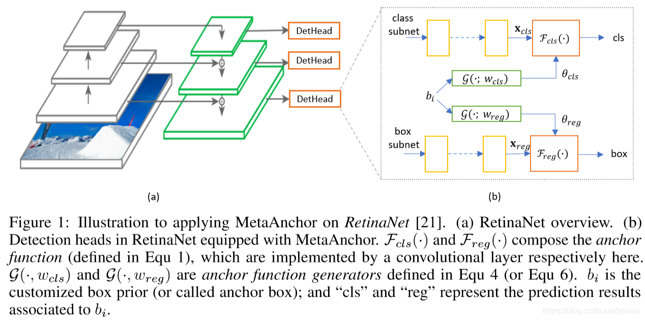
作者主要说明了MetaAnchor在RetinaNet上的使用,先来看看什么是RetianNet,放上一段简介的代码
class RetinaNet(nn.Module):
    num_anchors = 9

    def __init__(self, num_classes=20):
        super(RetinaNet, self).__init__()
        self.fpn = FPN50()
        self.num_classes = num_classes
        self.reg_head = self._make_head(self.num_anchors*4)
        self.cls_head = self._make_head(self.num_anchors*self.num_classes)

    def forward(self, x):
        fms = self.fpn(x)
        reg_preds = []
        cls_preds = []
        for fm in fms:
            loc_pred = self.loc_head(fm)
            cls_pred = self.cls_head(fm)
            loc_pred = loc_pred.permute(0,2,3,1).contiguous().view(x.size(0),-1,4)                 # [N, 9*4,H,W] -> [N,H,W, 9*4] -> [N,H*W*9, 4]
            cls_pred = cls_pred.permute(0,2,3,1).contiguous().view(x.size(0),-1,self.num_classes)  # [N,9*20,H,W] -> [N,H,W,9*20] -> [N,H*W*9,20]
            loc_preds.append(loc_pred)
            cls_preds.append(cls_pred)
        return torch.cat(loc_preds,1), torch.cat(cls_preds,1)

    def _make_head(self, out_planes):
        layers = []
        for _ in range(4):
            layers.append(nn.Conv2d(256, 256, kernel_size=3, stride=1, padding=1))
            layers.append(nn.ReLU(True))
        layers.append(nn.Conv2d(256, out_planes, kernel_size=3, stride=1, padding=1))
return nn.Sequential(*layers)
注: 以上代码来自于kuangliu/pytorch-retinanet
从以上代码
_make_head(self, out_planes)
函数中可以得知:我们必须把anchor的数量考虑并体现在RetinaNet最后一层卷积核的通道数量上。
那么作为RetinaNET网络结构的这个卷积核部分,就包含了我先验的一种设计(Anchor类型数为9)。
这样做的弊端就是:假如我换了anchor的种类或数量,那么就要重新改变这个卷积核的设计,进而影响了网络的结构和参数学习,那么这就意味着我先前学习的对于9个Anchor的RetinaNet不再具有一般性,不再具备迁移学习的能力。
如果我想,换一种数据集bbox的分布,或者换一种先验anchor的选择方式,网络依旧能够使用的话,就必须将anchor的先验从原来的设计中剥离出来作为一个独立的结构,从而不影响整体结构的设计,并且可以根据需求自定义不同的anchor设计,这也就是这篇论文要解决的问题,并冠以“MetaAnchor”的称号,并使用了一个$\mathcal{G}(b_i; w)$的anchor function generator
在RetianNet 的原设计中,每个detection head模块最后一层,对于预定义的3x3中anchor bboxes ,anchor function中:
- cls模块用3x3x80(类别)=720个通道卷积核,生成720维的预测向量
- reg模块有3x3x4=36个通道卷积核,生成36维的预测向量
而在使用MetaAnchor后,就降成了:
- cls模块有80(类别)=80个通道卷积核,生成80维的预测向量
- reg模块有4个通道卷积核,生成4维的预测向量
这就就需要重新设计anchor function。根据自己定制(customized)的anchor bbox${b_i}$首先,应该考虑如何编码${b_i}$,它包含了位置、尺寸、类别信息,多亏了RetianNet的全卷积结构,位置坐标信息已经包含在Feature map 中,我们使用$\mathcal{G}(\cdot)$来预测类别,那么${b_i}$只需要包含尺寸信息:
在一个训练的mini-batch中,我们给定一个二维$b_i$的数值,分别经过两层的全连接网络$\mathcal{G}(b_i; w_{cls})$和$\mathcal{G}(b_i; w_{reg})$的映射,得到一个$W_{cls}$和$W_{reg}$维度的参数$\theta_{cls,b_i}$和$\theta_{reg,b_i}$
论文里面没有给出这个参数$\theta_{cls,b_i}$和$\theta_{reg,b_i}$如何写入到Loss function中,我根据作者思路猜测:
论文提到$\mathcal{G} \left(b_i, w\right)$是一个低秩的子空间
不过根据论文的权重预测的思想,这里的参数$\theta_{cls,b_i}$和$\theta_{reg,b_i}$应该在lossfunction中发挥权重的作用,在训练过程中,通过给定一个位置和尺度下的anchor bbox的输出和标签,乘以相应权重,来计算该anchor点对应的所有anchors总的loss:
import torch
import numpy as np
import torch.nn.functional as F

def Anchor_bbox_size(ah_i,aw_i,level):
        minimum_size = 20
        AH,AW = minimum_size * np.pow(2,level-1)
        b_i=(np.log(ah_i/AH),np.log(aw_i/AW))
        return b_i

def anchor_bbox_generator(b_i,level=1):
    '''b_i = (log(ah_i/AH),log(aw_i/AW))
       b_t = [N,2]     '''

    hidden_dim = 5
    theta_dim = 10
    theta_standard =torch.randn(theta_dim)

    ## two -layer
    Residual_theta =F.linear( F.relu (F.linear(bi,(2,hidden_dim))) , (hidden_dim,theta_dim ) )

    theta_b_i = theta_standard + Residual_theta

    reutrn theta_b_i

class RetinaNet(nn.Module):

    def __init__(self, num_classes=20):
        super(RetinaNet, self).__init__()
        self.fpn = FPN50()
        self.num_classes = num_classes
        self.reg_head = self._make_head(4)
        self.cls_head = self._make_head(self.num_classes)

    def forward(self, x):
        fms = self.fpn(x)
        reg_preds = []
        cls_preds = []
        for fm in fms:
            loc_pred = self.loc_head(fm)
            cls_pred = self.cls_head(fm)
            loc_pred = loc_pred.permute(0,2,3,1).contiguous().view(x.size(0),-1,4)            # [N, 4,H,W] -> [N,H,W, 4] -> [N,H*W, 4]
            cls_pred = cls_pred.permute(0,2,3,1).contiguous().view(x.size(0),-1,self.num_classes)  # [N,20,H,W] -> [N,H,W,20] -> [N,H*W,20]
            loc_preds.append(loc_pred)
            cls_preds.append(cls_pred)
        return torch.cat(loc_preds,1), torch.cat(cls_preds,1)

    def _make_head(self, out_planes):
        layers = []
        for _ in range(4):
            layers.append(nn.Conv2d(256, 256, kernel_size=3, stride=1, padding=1))
            layers.append(nn.ReLU(True))
        layers.append(nn.Conv2d(256, out_planes, kernel_size=3, stride=1, padding=1))
return nn.Sequential(*layers)

def focal_loss_meta(bi,cls_pred,cls_label,reg_pred,reg_label):
    '''
    bi = [N,2]
    cls_pred = [N,20]
    cls_label = [N,]
    reg_pred = [N,4]
    reg_label = [N,4]

    '''


    alpha = 0.25
    gamma = 2
    num_classes = 20

    t = torch.eye(num_classes+1)(cls_label, )  # [N,21] 20+背景
    # t is one-hot vector
    t = t[:,1:]  # 去掉 background 【N,20】


    p = F.logsigmoid(cls_pred)
    pt = p*t + (1-p)*(1-t)         # pt = p if t > 0 else 1-p
    m = alpha*t + (1-alpha)*(1-t)
    m = m * (1-pt).pow(gamma)   # focal loss 系数 解决样本不平衡

    weight = anchor_bbox_generator(bi,) # [N,W] W维的θ参数,该怎么用? 还是说这里W=1??

    cls_loss = F.binary_cross_entropy_with_logits(x, t, m, size_average=False)
以上代码仅代表个人对论文的局限理解
因为看不到论文的代码,目前我理解最模糊的就是这个θ参数如何与loss function相结合的地方了,还请网友多多交流,欢迎发表更多的见解~
以上基本就介绍了是论文最主要的想法:
- MetaAnchor对于anchor的设定和bbox的分布更加鲁棒
- MetaAnchor可以缩减不同数据集bbox分布的差异的影响,即更具迁移学习的能力!
论文的更多的实验细节,我会继续阅读并更新博客~
=========================================
上次博客中说道,我理解最模糊的就是这个θ参数如何与ancnhor 的 loss function相结合的地方了
我重新阅读了论文,作者提到了权重预测的主要受到HyperNetworks的启发,然后我找来这篇论文,刚读完摘要,就恍然大悟理解了MetaAnchor里预测权重的思想,即这个θ参数的内涵,$\theta_{b_i}$ 即 $\mathcal{F}_{csl}\left(\cdot\right)$ 和 $\mathcal{F}_{reg}\left(\cdot\right)$的中的参数,在RetinaNet中代表了最后一层卷积核的参数!
原来我在这个点上理解困难的原因是头脑中少了“HyperNetworks”的先验!
看来很多情况下,我们理解的困难源于:少了某些“先验知识”
HyperNetwork (ICLR2017)
HyperNetwork是什么呢,简言之:
用一个网络(A-HyperNetwork)生成另外另一个网络(B-主体网络)的权重
听起来很神奇,因为我们一般对于网络B的学习,通常经过梯度下降法产生梯度来更新参数。而这个工作可以直接用另一个网络的输出来预测。这样做的好处就是,我们可以将巨大参数量的权重学习,转换为一个小网络的参数学习,并可以通过端到端梯度优化的方法学习!
这篇论文分析了LSTM和CNN使用HyperNetwork的方法和效果,结合我们主要论述的MetaAnchor,我来简要介绍一下Static HyperNetwork在CNN中的应用
通过一个两层全连接的小网络,用一个layer embedding来预测(表征)CNN的卷积核参数值
对于一个深度的卷积神经网络,其参数主要由卷积核构成
每个卷积核有 $N_{in} \times N_{out}$ 个滤波器 每个滤波器有 $f_{size} \times f_{size}$.
假设这些参数存在一个矩阵 $K^j \in \mathbb{R}^{N_{in}f_{size} \times N_{out}f_{size}}$ for each layer $j = 1,..,D$, 其中 $D$ 是卷积网络的深度
对于每一层 $j$, hypernetwork 接受一个 a layer embedding $z^j \in \mathbb{R}^{N_{z}}$ 作为输入,并预测 $K^j$, 可以写成:
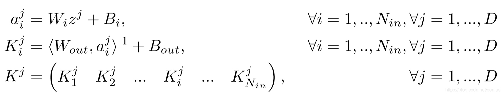
公式中,所有可学习的参数 $W_i$, $B_i$, $W_{out}$, $B_{out}$ 对于所有 $z^{j}$共享
在推理时, 模型仅仅将学习到的 the layer embeddings $z^j$ 来生成第 $j$ 层的卷积核权重参数
这就将可学习的参数量改变了:
应用到MetaAnchor中:$\theta_{b_i}$即RetinaNet的最后一层卷积核的参数
即,我们用自定义anchor设计${b_i}$成二维向量,作为“layer embedding”,输入两层的网络,预测了RetinaNet的最后一层卷积核参数的残差,这样就降低了原RetinaNet的卷积核滤波器的数量,就像之前提到的。
好了,我基本都搞清楚了,你呢
后面会继续贴出复现代码~